Sharding Overview

This page describes how MBIRJAX spreads a single reconstruction across several devices. It is a developer-oriented overview of the architecture – enough to follow how the pieces fit together and where they live in the code, not a line-by-line specification. For the user-facing view (how to turn it on and control it), see Multi-GPU Reconstruction.

Scope. Sharding runs within a single process across the available devices (multiple GPUs, or, with no GPU, multiple CPU devices). It works for every geometry and for the QGGMRF denoiser. A key invariant is that the result is independent of the number of devices: when a count does not divide evenly the data is zero-padded to equal shares and the padding is kept exactly inert. Multi-node execution is out of scope.

The two shardings

MBIRJAX shards the two large arrays along complementary axes:

• the reconstruction is sharded by slice – each device (a slice-owner) holds a contiguous band of slices of the voxel cylinders, (num_pixels, slices_per_device);

• the sinogram is sharded by view – each device (a view-owner) holds a block of views and is responsible for producing all detector rows for those views.

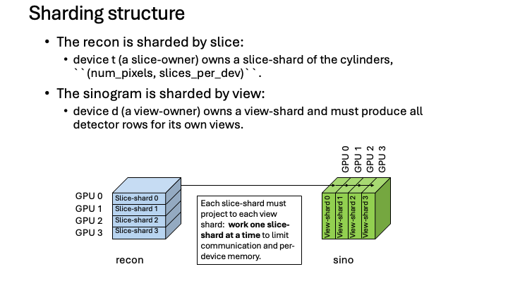
The recon is sharded by slice (left); the sinogram by view (right). Every slice-shard must reach every view-shard, so projection is an all-to-all between the two layouts.

Because the two arrays are sharded on different axes, projecting between them is an all-to-all: every slice-shard contributes to every view-shard, and vice versa. To bound both the inter-device communication and the peak per-device memory, the projectors work one slice-shard at a time rather than moving the whole volume at once.

Placement: the single source of device layout

Device layout is described by a single object, Placement (in mbirjax/_sharding/placement.py). A placement records:

• the list of devices;

• which array axis is sharded;

• the real_size of that axis and the padded_size (rounded up to a multiple of the device count);

• its own 1-D mesh.

A model carries two placements – recon_placement (slice axis) and sino_placement (view axis) – and these are the single source of truth for where every array lives; there is no separate “main device” or “is-sharded” state.

Automatic selection uses all available devices – occasionally fewer, in the unusual case where an extra device would do no useful work (the exact policy is a tunable heuristic). Padding is exactly inert (entry zero-fill, projector output masks, and the prior-interface mask all keep it from affecting any result), which is what makes the output independent of the device count. For explicit control, see configure_devices().

Forward and back projection by bands

Within a slice-shard the work is subdivided once more, into bands of slices. Both projectors run a double loop: over slice-shards (outer) and over bands (inner). Banding bounds the size of the transient buffers that arise while moving data between the two shardings.

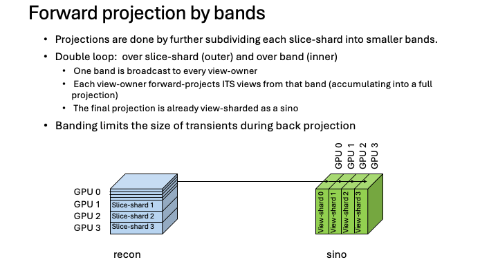
Forward projection: one band is broadcast to every view-owner, each view-owner forward-projects its own views from that band (accumulating), and the result is already a view-sharded sinogram.

Forward projection (recon → sinogram) broadcasts each band to every view-owner; each view-owner forward-projects its own views from that band and accumulates into its part of the sinogram. When the loop finishes, the sinogram is already in the view-sharded layout.

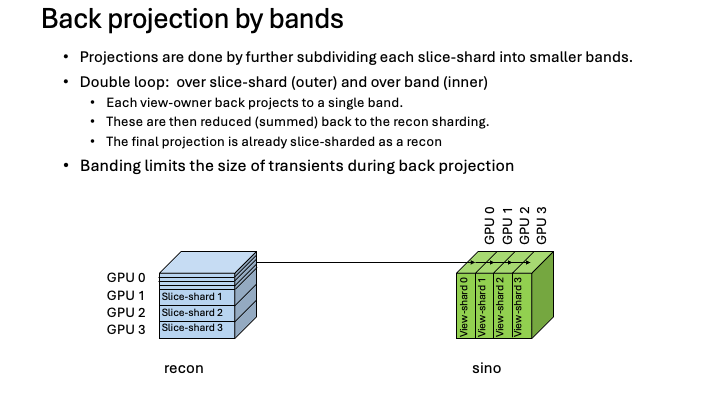
Back projection: each view-owner back-projects to a single band; the contributions are reduced (summed) over views into the recon’s slice sharding.

Back projection (sinogram → recon) is the adjoint: each view-owner back-projects into a band, and the per-view contributions are reduced (summed) and scattered into the slice-owner that holds those slices – a reduce-scatter. The result is already in the slice-sharded recon layout.

Why cone beam projects whole cylinders

In parallel-beam geometry detector row r maps only to slice r with no cross-row mixing, so a device can produce just the slices a destination needs by first slicing its sinogram views to those rows – the transient cylinder buffer can be held at one destination’s slice range.

Cone beam cannot do this cheaply: magnification maps a single slice to a data-dependent band of detector rows (dependent on the cone angle and the particular slice), so the slice and detector-row axes are coupled. This projection could proceed one band of slices at a time, but then each detector row requires multiple updates from a single voxel cylinder. Alternatively, each view owner can collect all the bands for a batch of pixels and then project the resulting full cylinders. A/B tests on representative shapes showed that the second approach increased transient memory for the projector by about 10% but decreased time by about 2x.

A view-owner therefore collects the full voxel cylinder once and then projects the full cylinder, rather than restricting the computation to a band up front. This coupling is also why the sinogram is sharded by view (not by detector row) uniformly across geometries.

The QGGMRF prior and halos

The QGGMRF prior is local: each voxel interacts only with its neighbors. Across slices that means a slice-owner can evaluate the prior on its own band entirely locally except at the boundary between two adjacent slice-shards, where it needs the neighbor’s boundary slice. Those boundary slices are exchanged as halos between neighboring owners. At the outer edge of the volume there is no neighbor, so the boundary condition is reflection; a single shard (one device) is reflected at both edges and needs no halos at all (_extract_halos / _stage_halos in tomography_model.py).

Halo staging happens host-side and so cannot live inside a JIT, which drives the single- vs multi-device split below.

Single- and multi-device paths

The prior-bearing loops (the VCD reconstruction and the denoiser) take one of two paths depending on the device count:

• One device – the whole sweep compiles into a single JIT. A single shard is reflected at both edges, so no halos are needed and there is no Python-level loop.

• Several devices – a Python loop runs the passes, staging the halos host-side once per pass (the part that cannot be jitted), and the on-device per-pass work stays compiled.

Both paths converge to the same result; only the boundary handling and the loop structure differ.

A related platform split exists for cone-beam back projection: the GPU single-device case uses a rolled-pixel kernel (back_project_one_view_to_pixel_batch), while CPU and the multi-device reduce-scatter use a band kernel (back_project_one_view_to_band). The two kernels have opposite platform rankings, so the driver selects by platform.

Multi-device execution: thread pools

The steps above all share a common substrate: run a kernel on each device, then combine the per-device outputs into one sharded array. Within a single step the per-device kernels are independent (each device works on its own shard or band); the cross-device communication – the broadcast in forward projection, the reduce-scatter in back projection – happens between steps, not inside them. The design problem is to launch those per-device kernels and reassemble their outputs without bouncing data through host memory, which the obvious approaches on GPU fail to do (they pay host-transfer cost or hit hardware-portability problems).

MBIRJAX uses a thread pool with one worker per device: each thread reads its shard in place (addressable_shards – the data is already resident on that device, so there is no host copy), runs the per-device kernel on its device, and keeps its result on-device. The per-device results are reassembled into one logically global, sharded jax.Array with jax.make_array_from_single_device_arrays – with no host round-trip in either direction (device_pool / run_per_device / assemble_sharded in mbirjax/_sharding/thread_execution.py).

The table below summarizes the approaches that were measured (full study with timings on H100, L40S, and CPU in experiments/sharding/parallel_performance/fbp_filter_parallelism_comparison.md):

Approach	Host (PCIe) transfer	Correctness	Verdict
Thread pool, fully on-device	none	correct on all hardware tested	used (≈2× on 2 GPUs)
shard_map (SPMD)	none	wrong on L40S (cause unknown); correct on H100	not hardware-safe
Threads, gather through host	fixed cost, independent of device count	correct	dominated by transfer
pmap	–	–	deprecated

The thread-pool approach was chosen because it transfers nothing through host memory, is correct on every device tested, and produces output already in the sharded layout the next step expects. shard_map is a viable future upgrade (slightly faster on H100) if the L40S correctness discrepancy is ever diagnosed.

Where this lives in the code

• mbirjax/_sharding/placement.py – the Placement object and array movement.

• mbirjax/_sharding/thread_execution.py – the thread-pool execution helpers.

• the per-geometry projector kernels (e.g. back_project_one_view_to_band) in parallel_beam.py / cone_beam.py / translation_model.py / multiaxis_parallel.py.

• denoising.py – the single-/multi-device denoiser paths.

The strongest correctness gate for the inert-padding invariant is the poison-the-padding test: a forward projection of a recon whose padded slices are nonzero must bit-match the clean-padded forward. Results are also checked against a single-device reference and across device counts.