
Utilities#
MBIRJAX contains utilities for viewing, downloading, exporting/importing, and generating synthetic data.
Saving and loading models and reconstructions is handled through TomographyModel: Saving and Loading.
3D Data Viewer#
- mbirjax.viewer.slice_viewer(*datasets, data_dicts=None, title='', vmin=None, vmax=None, slice_label=None, slice_axis=None, cmap='gray', show_instructions=True)[source]#
Launch an interactive viewer for inspecting one or more 2D or 3D image arrays.
This function provides a graphical interface for exploring one or more 3D volumes or 2D slices. Features include synchronized slice navigation, ROI statistics, axis transposition, file loading, dynamic intensity range adjustment, and interactive GUI tools for zooming and panning.
Each image can have an associated data dict, typically obtained from
TomographyModel.recon(), which can be viewed as a text file within the viewer.Designed primarily for inspecting CT or other volumetric reconstructions in research workflows.
- Parameters:
*datasets (ndarray or None) – One or more 2D or 3D NumPy arrays to display. - 2D arrays are automatically promoted to 3D via a singleton axis. - None values are replaced with placeholder zero arrays.
data_dicts (None or dict or list of None or dicts, optional) – Dictionary of string entries to associated with the data (e.g., from
TomographyModel.get_recon_dict())title (str, optional) – Window title. Defaults to an empty string.
vmin (float, optional) – Minimum intensity value for display. Defaults to the global minimum across all datasets.
vmax (float, optional) – Maximum intensity value for display. Defaults to the global maximum across all datasets.
slice_label (str or list of str, optional) – Label(s) for the current slice. Defaults to “Slice”.
slice_axis (int or list of int, optional) – Axis along which to slice (0, 1, or 2). Defaults to the last axis (2).
cmap (str, optional) – Colormap to use. Defaults to “gray”.
show_instructions (bool, optional) – Whether to display usage instructions in the figure. Defaults to True.
Notes
This function blocks execution until the viewer window is closed.
Right-click an image to access a context menu with options such as axis transposition and file loading.
Right-click the intensity slider (if using TkAgg backend) to manually set display range bounds.
Press ‘h’ to show help overlay. Press ‘Esc’ to clear overlays or reset ROI selections.
Example
>>> denoiser = mj.QGGMRFDenoiser(noisy_image.shape)
>>> denoised_image, denoised_dict = denoiser.denoise(noisy_image)  # Estimate the noise level from the image
>>> mj.slice_viewer(noisy_image, denoised_image, data_dicts=[None, denoised_dict], title='Noisy and denoised images')
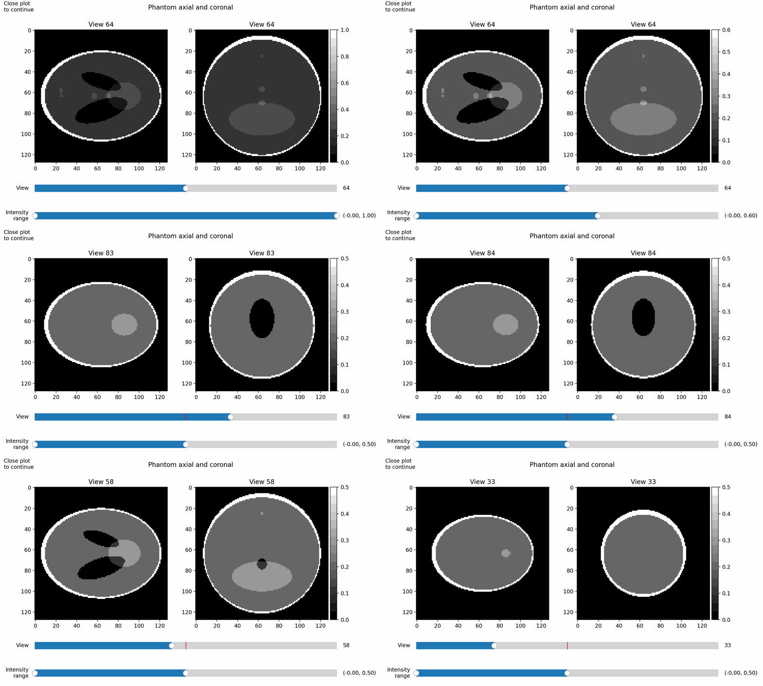
Here is an example showing views of a modified Shepp-Logan phantom, with changing intensity window and displayed slice:
General Purpose#
- mbirjax.utilities.stitch_arrays(array_list, overlap, axis=2, ramp_overlap=None)[source]#
Concatenate JAX arrays along one axis while linearly blending a fixed overlap between adjacent arrays.
This behaves like jnp.concatenate except that for each adjacent pair, the first overlap_length elements of the second array and the last overlap_length elements of the current result are combined by a piece-wise linear cross‑fade.
All non‑axis dimensions must match across inputs.
- Parameters:
array_list (list of ndarray or jax.Array) – Sequence of 2+ arrays to stitch. The result is built on the inputs’ own array module, so host (NumPy) inputs stitch on the host (no gather to a single device) and jax inputs stitch on-device.
overlap (int) – Number of elements overlapped between arrays. Must be >= 1 and not exceed the length of any input along axis.
axis (int, optional) – Axis along which to stitch. Defaults to 2.
ramp_overlap (int, optional) – Target number of blended (0 < w < 1) elements. Defaults to None.
- Returns:
ndarray or jax.Array – Stitched array, on the inputs’ own array module (host NumPy in -> host out, jax in -> on-device out). Its shape equals the input shape with the length along axis equal to:
sum(len_k) - (len(array_list) - 1) * overlap_length
where len_k are the lengths of each input along axis.
- Raises:
ValueError – If fewer than two arrays are provided, if non‑axis dimensions differ, or if any array is shorter than overlap_length along axis.
Example
>>> import jax.numpy as jnp
>>> a0 = jnp.arange(2*2*5).reshape(2, 2, 5)
>>> a1 = jnp.arange(2*2*6).reshape(2, 2, 6)
>>> out = stitch_arrays([a0, a1], overlap=3, axis=2)
>>> out.shape
(2, 2, 8)
# 8 comes from 5 + 6 - 3 (one overlap between two arrays).
- mbirjax.utilities.get_ct_model(geometry_type, sinogram_shape, angles, source_detector_dist=None, source_iso_dist=None, helical_z_shifts=None)[source]#
Create an instance of TomographyModel with the given parameters
- Parameters:
geometry_type (str) – ‘parallel’ or ‘cone’
sinogram_shape (tuple list of int) – (num_views, num_rows, num_channels)
angles (ndarray of float) – 1D vector of projection angles in radians
source_detector_dist (float or None, optional) – Distance in ALU from source to detector. Defaults to None for geometries that don’t need this.
source_iso_dist (float or None, optional) – Distance in ALU from source to iso. Defaults to None for geometries that don’t need this.
helical_z_shifts (numpy or jax array, optional) – Per-view axial shifts (ALU), same length as angles. Required when use_helical=True.
- Returns:
An instance of ConeBeamModel or ParallelBeam model
- mbirjax.utilities.copy_ct_model(ct_model, new_angles=None, new_helical_z_shifts=None, new_num_det_rows=None, new_num_det_cols=None)[source]#
Create a TomographyModel with the same type and parameters as the given ct_model except with the new input angles and a corresponding sinogram shape. Restricted to ParallelBeam and ConeBeam models.
- Parameters:
ct_model (TomographyModel) – The model to copy.
new_angles (ndarray of float, optional) – 1D vector of projection angles in radians. If None, then use the angles in ct_model. Defaults to None.
new_helical_z_shifts (ndarray of float, optional) – 1D vector of per-view axial shifts in ALU for ConeBeamModel. Defaults to None.
new_num_det_rows (int, optional) – Number of detector rows in the new model. If None, then use the num_det_rows in ct_model. Defaults to None.
new_num_det_cols (int, optional) – Number of detector columns in the new model. If None, then use the num_det_cols in ct_model. Defaults to None.
- Returns:
An instance of ConeBeamModel or ParallelBeam model
Weight Generation#
- mbirjax.vcd_utils.gen_weights(sinogram, weight_type, ct_model=None)[source]#
Compute optional weights used in MBIR reconstruction based on the noise model.
The weights should be proportional to the inverse variance of the noise for each sinogram entry. They can be used to improve reconstruction quality.
The result is returned where the input lives, so it feeds reconstruction without landing a large array on a single device:
a host (NumPy) sinogram yields host weights (reconstruction streams them to the devices shard-by-shard);
a JAX array yields JAX weights inheriting its sharding (a view-sharded sinogram gives view-sharded weights, with no cross-device communication or gather).
To build the weights already distributed across a multi-device reconstruction – avoiding any single-device copy of a large host sinogram – pass the model as
ct_model: the sinogram is placed in the model’s view-sharded device form first, then weighted per shard.- Parameters:
sinogram (ndarray or jax.Array) – A 3D array of shape (num_views, num_det_rows, num_det_channels) representing the sinogram.
weight_type (str) – The type of noise model to use for weighting. Must be one of: - ‘unweighted’: Use uniform weights (all ones). - ‘transmission’: Use exponential decay, exp(-sinogram). - ‘transmission_root’: Use square-root decay, exp(-sinogram / 2). - ‘emission’: Use reciprocal decay, 1 / (abs(sinogram) + 0.1).
ct_model (TomographyModel, optional) – If given, distribute the sinogram in this model’s sinogram device form (view-sharded across its devices) before weighting, so the weights are returned sharded and ready for reconstruction with no single-device copy. Defaults to None (the result preserves the input’s residence, as described above).
- Returns:
ndarray or jax.Array – A 3D array of weights with the same shape as the input sinogram, on the host or sharded across devices to match the input (or
ct_model).- Raises:
Exception – If weight_type is not one of the supported options.
Note
For transmission noise models, sinogram values should not be excessively large (e.g., > 5), as this corresponds to near-zero transmission, which is not physically meaningful in typical X-ray imaging.
Example
>>> sinogram = jnp.ones((180, 64, 128))
>>> weights = gen_weights(sinogram, weight_type='transmission_root')
>>> weights.shape
(180, 64, 128)
- mbirjax.vcd_utils.gen_weights_mar(ct_model, sinogram, init_recon=None, metal_threshold=None, beta=1.0, gamma=3.0)[source]#
Generates the weights used for reducing metal artifacts in MBIR reconstruction.
This function computes sinogram weights that help to reduce metal artifacts. More specifically, it computes weights with the form:
weights = exp( -(sinogram/beta) * ( 1 + gamma * delta(metal) ) )
delta(metal) denotes a binary mask indicating the sino entries that contain projections of metal. Providing
init_reconyields better metal artifact reduction. If not provided, the metal segmentation is generated directly from the sinogram.- Parameters:
sinogram (jax array) – 3D jax array containing sinogram with shape (num_views, num_det_rows, num_det_channels).
init_recon (jax array, optional) – An initial reconstruction used to identify metal voxels. If not provided, Otsu’s method is used to directly segment sinogram into metal regions.
metal_threshold (float, optional) – Values in
init_reconabovemetal_thresholdare classified as metal. If not provided, Otsu’s method is used to segmentinit_recon.beta (float, optional) – Scalar value in range \(>0\). A larger
betaimproves the noise uniformity, but too large a value may increase the overall noise level.gamma (float, optional) – Scalar value in range \(>=0\). A larger
gammareduces the weight of sinogram entries with metal, but too large a value may reduce image quality inside the metal regions.
- Returns:
(jax array) – Weights used in mbircone reconstruction, with the same array shape as
sinogram
IO Functions#
As noted above, saving and loading models and reconstructions is handled through TomographyModel: Saving and Loading.
The functions here are for direct interactions with files.
- mbirjax.utilities.download_and_extract(download_url, save_dir)[source]#
Download or copy a file from a URL or local file path. If the file is a tarball (.tar, .tar.gz, etc.), extract it into the specified directory. Supports Google Drive links, standard HTTP/HTTPS URLs, and local paths.
If the file already exists in the save directory, it will not be re-downloaded or copied.
- Parameters:
download_url (str) – URL or local file path to the file. Supported formats include: - Google Drive shared links - HTTP/HTTPS URLs - Local file paths
save_dir (str) – Directory where the file will be saved and extracted (if applicable).
- Returns:
str – - For tar files: Path to the extracted top-level directory. - For other files: Path to the downloaded or copied file.
- Raises:
RuntimeError – If the file cannot be downloaded, copied, or extracted.
ValueError – If the Google Drive URL is invalid or tar file has no top-level directory.
Examples
>>> extracted_dir = download_and_extract("https://example.com/data.tar.gz", "./data")
>>> file_path = download_and_extract("https://drive.google.com/file/d/1ABC123/view", "./data")
>>> result = download_and_extract("/path/to/local/data.tar.gz", "./data")
- mbirjax.utilities.save_data_hdf5(file_path, array, array_name='array', attributes_dict=None)[source]#
Save a NumPy or JAX array to an HDF5 file, optionally including metadata as attributes. The resulting structure has a single dataset with one array and associated text attributes. These can be retrieved using
load_data_hdf5().- Parameters:
file_path (str) – Full path to the output HDF5 file. Directories will be created if they do not exist.
array (ndarray or jax.Array) – The volume data to save.
array_name (str) – Name of the dataset within the HDF5 file. Defaults to ‘array’.
attributes_dict (dict, optional) – Dictionary of attributes to store as metadata in the dataset. Keys must be strings, and values should be serializable as HDF5 attributes.
- Returns:
None
Example
>>> import numpy as np
>>> volume = np.random.rand(64, 64, 64)
>>> attrs = {'voxel_size': '1.0mm', 'modality': 'CT'}
>>> save_data_hdf5('output/recon.h5', volume, array_name='recon', attributes_dict=attrs)
Nothing
Example
>>> recon, recon_dict = ct_model.recon(sinogram)
>>> recon_info = {'ALU units': '0.3mm', 'sinogram name': 'test part 038'}
>>> file_path = './output/test_part_038.yaml'
>>> mj.save_data_hdf5(file_path, recon, recon_info)
- mbirjax.utilities.load_data_hdf5(file_path)[source]#
Load a numpy array from an HDF5 file.
This function loads an array stored in an HDF5 file using
save_data_hdf5(). It also loads any associated attributes and returns them as a dict.- Parameters:
file_path (str) – Path to the HDF5 file containing the reconstructed volume.
- Returns:
tuple –
- (array, data_dict)
array (ndarray): The array saved by
save_data_hdf5()data_dict (dict): A dict with the attributes for the data array.
- Raises:
FileNotFoundError – If the file does not exist.
ValueError – If more than one dataset is not found in the file.
Example
>>> import mbirjax as mj
>>> recon, recon_dict = mj.load_data_hdf5("output/recon_volume.h5")
>>> recon.shape
(64, 256, 256)
- mbirjax.utilities.export_recon_hdf5(file_path, recon, recon_dict=None, remove_flash=False, radial_margin=10, top_margin=10, bottom_margin=10)[source]#
Export a 3D reconstruction volume to an HDF5 file with optional post-processing.
This function works with either numpy or jax arrays or sharded jax arrays. The function also transposes the reconstruction to right-hand coordinates (slice, col, row), and writes the reconstruction and optional metadata to an HDF5 file.
- Parameters:
file_path (str) – Full path to the output HDF5 file. Parent directories will be created if they do not exist.
recon (Union[np.ndarray, jax.Array]) – 3D volume in (row, col, slice) order. Will be converted to NumPy before writing.
recon_dict (dict, optional) – Dictionary of attributes to store as metadata in the dataset.
remove_flash (bool, optional) – Whether to apply a cylindrical mask to remove peripheral and top/bottom slices. Defaults to False.
radial_margin (int, optional) – Margin in pixels to subtract from the cylinder radius. Defaults to 10.
top_margin (int, optional) – Number of top slices to set to zero along the Z-axis. Defaults to 10.
bottom_margin (int, optional) – Number of bottom slices to set to zero along the Z-axis. Defaults to 10.
Example
>>> from mbirjax.utilities import export_recon_hdf5
>>> import jax.numpy as jnp
>>> recon = jnp.ones((128, 128, 64))  # (row, col, slice) order
>>> export_recon_hdf5("output/recon_volume.h5", recon, recon_dict={"scan_id": "sample1"})
- mbirjax.utilities.import_recon_hdf5(file_path)[source]#
Import a 3D reconstruction volume from an HDF5 file.
This function loads a reconstruction volume and associated metadata from an HDF5 file, and reorders the volume axes from the file’s (slice, col, row) layout to (row, col, slice) to match MBIRJAX conventions, so a volume written by export_recon_hdf5 is recovered unchanged.
- Parameters:
file_path (str) – Path to the HDF5 file containing the reconstruction volume.
- Returns:
Tuple[np.ndarray, dict] –
- A tuple containing:
recon (np.ndarray): The reconstructed 3D volume in (row, col, slice) order.
recon_dict (dict): Dictionary containing metadata associated with the reconstruction.
Example
>>> from mbirjax.utilities import import_recon_hdf5
>>> recon, recon_dict = import_recon_hdf5("output/recon_volume.h5")
>>> print(recon.shape)
(128, 128, 64)
Synthetic Data Generation#
- mbirjax.utilities.generate_demo_data(object_type: ObjectType | str = ObjectType.SHEPP_LOGAN, model_type: ModelType | str = ModelType.CONE, num_views: int = 64, num_det_rows: int = 96, delta_det_row: float = 1, num_det_channels: int = 128, delta_det_channel: float = 1, num_x_translations: int = 7, num_z_translations: int = 7, x_spacing: float = 22, z_spacing: float = 22, use_helical: bool = False, helical_pitch: float | None = None, helical_z_range: float | None = None, helical_z_center: float = 0.0, use_curved_detector: bool = False, voxel_row_aspect: float = 1.0, voxel_slice_aspect: float = 1.0, target_max_attenuation: float | None = None, devices: list | tuple | None = None) tuple[source]#
Create a simple object and a sinogram for demonstration purposes.
This function will create a 3D volume (aka object or phantom) of the specified type, then use the model type and parameters to create a simulated sinogram. The object type ‘shepp-logan’ gives a simplified version of the classic Shepp-Logan test phantom, and type ‘cube’ gives a simple cube object.
The phantom and the sinogram are built distributed across the model’s devices (in parallel) so a large problem is never materialized whole on one device, then gathered to the host: both are returned on the host. The output sinogram has shape (num_views, num_det_rows, num_det_channels); each 2D array sinogram[view_index] is a simulated image from the detector, with num_det_rows indicating the vertical size and num_det_channels the horizontal size.
- Parameters:
object_type (str, optional) – One of ‘shepp-logan’ or ‘cube’. Defaults to ‘shepp-logan’.
model_type (str, optional) – One of ‘parallel’, ‘cone’, or ‘translation’. Defaults to ‘cone’.
num_views (int, optional) – Number of views in the output sinogram. Defaults to 64. Ignored when model_type is ‘translation’
num_det_rows (int, optional) – Number of rows (vertical) in the output sinogram. Defaults to 96.
num_det_channels (int, optional) – Number of channels (horizontal) in the output sinogram. Defaults to 128.
num_x_translations (int, optional) – Number of horizontal translations for translation mode. Defaults to 7.
num_z_translations (int, optional) – Number of vertical translations for translation mode. Defaults to 7.
x_spacing (float, optional) – Horizontal spacing between translations in ALU. Defaults to 22.
z_spacing (float, optional) – Vertical spacing between translations in ALU. Defaults to 22.
use_helical (bool, optional) – If True and model_type == ‘cone’, generate a helical cone-beam trajectory by supplying per-view z_shifts to ConeBeamModel. Defaults to False.
helical_pitch (float, optional) – Helical pitch (dimensionless) for helical mode. pitch = (table travel per rotation) / (det height at iso). This is the fraction of the detector height at iso traveled per rotation.
helical_z_range (float, optional) – Total axial travel over the scan in ALU for helical mode.
helical_z_center (float, optional) – Midpoint of axial travel over the scan in ALU for helical mode.
use_curved_detector (bool, optional) – (cone beam geometry parameter)
voxel_row_aspect (float, optional) – Aspect ratio for recon rows relative to columns. Defaults to 1.0.
voxel_slice_aspect (float, optional) – Aspect ratio for recon slices relative to rows. Defaults to 1.0.
target_max_attenuation (float, optional) – Target max sinogram attenuation for Shepp-Logan phantom. Defaults to None, for which each voxel is in the range [0, 1]. May not be accurate if any detector or voxel dimensions are not 1.
devices (sequence of jax devices, optional) – Devices to distribute the generation across. Defaults to None, which uses the model’s automatic selection (all available GPUs, else the CPU devices). The phantom and sinogram are built across these devices in parallel and then gathered to the host – this only affects where the work runs, not the result.
- Returns:
tuple –
- (object, sinogram, params)
object: the phantom volume, shape recon_shape = (num_rows, num_cols, num_slices).
sinogram: shape (num_views, num_det_rows, num_det_channels).
params (dict): contains ‘angles’ and, for ‘cone’, also ‘source_detector_dist’ and ‘source_iso_dist’.
sinogram is always a host NumPy array (what
reconprefers – it shards it across devices itself), and the arrays inparamsare NumPy as well. object is host NumPy for ‘shepp-logan’ but a JAX array for ‘cube’.
- mbirjax.utilities.generate_3d_shepp_logan_reference(phantom_shape)[source]#
Generate a 3D Shepp Logan phantom based on below reference.
Kak AC, Slaney M. Principles of computerized tomographic imaging. Page.102. IEEE Press, New York, 1988. https://engineering.purdue.edu/~malcolm/pct/CTI_Ch03.pdf
- Parameters:
phantom_shape (tuple or list of ints) – num_rows, num_cols, num_slices
- Returns:
out_image – 3D array, num_slices*num_rows*num_cols
Note
This function produces 6 intermediate arrays that each have shape phantom_shape, so if phantom_shape is large, then this will use a lot of peak memory.
- mbirjax.utilities.generate_3d_shepp_logan_low_dynamic_range(phantom_shape, devices=None, max_block_gb=4.0, target_max_attenuation=None)[source]#
Generates a 3D Shepp-Logan phantom with specified dimensions.
The phantom is a reference object, so it is always returned as a host NumPy array: the build is distributed across
devices(slice-sharded, in parallel) so a large phantom is never materialized whole on a single device, then it is gathered to the host and the device arrays are freed.- Parameters:
phantom_shape (tuple) – Phantom shape in (rows, columns, slices).
devices (sequence of jax devices, optional) – Devices to build the phantom across. Defaults to None, which uses all available devices (the GPUs when a GPU backend is present, else the CPU devices) – the same set a reconstruction would shard over. With more than one device the phantom is built slice-sharded (each device builds its own band of slices, no inter-device communication); with a single device it is built row-blocked to bound peak memory. Either way the result is gathered to the host.
max_block_gb (float, optional) – Rough upper bound (GB) on the temporary memory used by the single-device (row-blocked) build. Defaults to 4.0. Ignored for a multi-device build (each device’s slice band is already small).
target_max_attenuation (float, optional) – If given, scale the phantom so that the peak line integral through it (its forward projection) is roughly this value, independent of the array shape. Without it, the sinogram grows linearly with the array size (a ray crosses more voxels), which is unrealistic – real -log-attenuation sinograms sit around 0 to 6-8. The scale is analytic (from the main ellipsoid’s extent along the longest axis) and ASSUMES
delta_voxel ~= 1, since the phantom cannot see the projector’s voxel spacing (the sinogram scales linearly withdelta_voxel). Default None leaves the phantom unscaled (the historical behavior).
- Returns:
numpy.ndarray – A 3D host array of shape
phantom_shapewith the voxel intensities of the phantom.
Note
The phantom is independent across voxels, so the multi-device build splits slices and the single-device build blocks rows – neither needs inter-device communication.
- mbirjax.utilities.gen_translation_phantom(recon_shape, option, text, fill_rate=0.05, font_size=20, text_row_indices=None, horizontal_offset=0, vertical_offset=0, voxel_slice_aspect=1.0)[source]#
Generate a synthetic ground truth phantom based on the selected option.
- Parameters:
recon_shape (tuple[int, int, int]) – Shape of the reconstruction volume.
option (str) – Phantom type to generate. Options are ‘dots’ or ‘text’.
text (list[str]) – List of ASCII text strings to render.
fill_rate (float, optional) – Fill rate of the reconstruction volume. Default is 0.05.
font_size (int, optional) – Font size of the ASCII words. Default is 20.
text_row_indices (list[int], optional) – List of row indices where each text string should be placed. Default is None. If None, words are automatically distributed evenly across the first dimension. Must have the same length as ‘words’ if provided.
horizontal_offset (int, optional) – Horizontal offset of the text to be rendered. Positive value shifts the phantom right. Default is 0.
vertical_offset (int, optional) – Vertical offset of the text to be rendered. Positive value shifts the phantom up. Default is 0.
voxel_slice_aspect (float, optional) – Ratio between slice voxel spacing and column voxel spacing. Default is 1.0.
- Returns:
np.ndarray – Generated phantom volume.